Nucleophile Substitution CH3Cl - Standard MD
Task
The main task of this example is to learn how to monitor distances on the example of a nucleophile substitution of a Cl- by another Cl- in CH3Cl.
Input
POSCAR
CH3Cl
   1.00000000000000
    12.0000000000000000    0.0000000000000000    0.0000000000000000
     0.0000000000000000   12.0000000000000000    0.0000000000000000
     0.0000000000000000    0.0000000000000000   12.0000000000000000
C H Cl
   1   3   2
cart
         5.91331371  7.11364924  5.78037960
         5.81982231  8.15982106  5.46969017
         4.92222130  6.65954232  5.88978969
         6.47810398  7.03808479  6.71586385
         4.32824726  8.75151396  7.80743202
         6.84157897  6.18713289  4.46842049
- The starting POSCAR file for this example can be found under POSCAR.init. It will be needed for the script that runs the job (run.sh).
- A sufficiently large cell is chosen to minimize the interactions between neighbouring cells and hence to simulate an isolated molecular reaction.
KPOINTS
Automatic
 0
Gamma
 1  1  1
 0. 0. 0.
- For isolated atoms and molecules interactions between periodic images are negligible (in sufficiently large cells) hence no Brillouin zone sampling is necessary.
INCAR
PREC=Low
EDIFF=1e-6
LWAVE=.FALSE.
LCHARG=.FALSE.
NELECT=22
NELMIN=4
LREAL=.FALSE.
ALGO=VeryFast
ISMEAR=-1
SIGMA=0.0516

############################# MD setting #####################################
IBRION=0                                           # MD simulation
NSW=1000                                           # number of steps
POTIM=1                                            # integration step
TEBEG=600                                          # simulation temperature
MDALGO=11                                          # metaDynamics with Andersen thermostat
ANDERSEN_PROB=0.10                                 # collision probability
##############################################################################
- Molecular dynamics are switched on by the tag IBRION=0.
- The metadynamics tag MDALGO=11 is only used to monitor the two C-Cl distances defined in the ICONST file.
- Simulations are carried out in the NVT ensemble at approximately room temperature (TEBEG=300) and the Andersen thermostat is used for the temperature control. The strength of the coupling is controlled by the collision probability ANDERSEN_PROB=0.10.
- The accuracy of this calculation is kept low (PREC=Low and ALGO=VeryFast), which is completely sufficient for this tutorial. For more quantitative results this tags should be investigated (of course at the cost of higher computational demand).
- A charged system (due to the "incoming" Cl-) is simulated, so the number of electrons is raised by one compared to the neutral system (NELECT=22). To compensate for the charge a positive homogeneous background charge is assumed.
- Although very light atoms are present in the structure (hydrogen) a time step of 1 fs (POTIM=1) is safe to use. This can be achieved by setting the mass of hydrogen to that of tritium (look for the line "POMASS = 3.016" in the POTCAR file). This is unproblematic since the free energy is independent of the mass of atoms.
ICONST
For this example an ICONST file is used which looks like:
R 1 5 0
R 1 6 0
S 1 -1 7
- First line: This line selects the interatomic distance (R) between the first (C) and the fifth atom (Cl) in the POSCAR file. The 0 at the fourth entry would usually specify that the distances are constrained but if the coordinates are used later for special coordinates the constraining is not applied (for further information see ICONST).
- Second line: Same as the first line but interatomic distance between the first (C) and the sixth atom (Cl) in the POSCAR file is selected.
- Third line: This line selects a linear combination (option S) of the first two coordinates where the second and fourth column specify the coefficients of the coordinates. The setting of 1 and -1 corresponds to the difference between both. The 7 at the fourth entry specifies that difference between these two distances is monitored but no constraints are applied.
Calculation
Running the calculation
We are chopping the "relatively" long calculation into smaller peaces. So after each step we have to save the output and copy the CONTCAR file to POSCAR file to restart the calculation. All of this is done by the script run provided with this example:
#run
runvasp="mpirun -np 8 executable_path/vasp_gam"
# make sure to always start with the same structure
cp POSCAR.init POSCAR

i=1

while [ $i -le 50 ]
do
  # start vasp
  $runvasp

  # use the last configuration generated in the previous
  # run as initial configuration for the next run
  cp CONTCAR POSCAR

  # backup some important files
  cp REPORT REPORT.$i
  cp vasprun.xml vasprun.xml.$i

  let i=i+1
done
The only thing the user has to provide is the path of the executable under "executable_path". After running the script with the command ./run we should obtain we should obtain 50 output files each for a 1000 fs run totalling to a trajectory of 50 ps. It should be mentioned that this can take several hours on 8 cores so if the user has only limited time and resources available or is only interested to learn the execution of this example the number of runs (line "[ $i -le 50 ]") can be changed from 50 to a smaller value. Also the number of timesteps per run can be lowered (NSW).
Time evolution of distance
- The monitored value of the distance between the two Cl- ions defined in the ICONST file is written for each molecular dynamics run to the REPORT file written as "mc = ...". The time evolution function of this variable is monitored using the script timeEv.sh:
#!/bin/bash

if test -f "timeEvol.dat"; then
   rm timeEvol.dat
fi

i=1
while [ $i -le 1000 ]
do
   if test -f REPORT.$i
   then
     grep mc REPORT.$i |awk '{print $3 }' >>timeEvol.dat
   fi
   let i=i+1
done
It creates a file "timeEvol.dat" holding the value for the collective variable at every molecular dynamics step.
- After that the task is to get a histogram (or probability distribution) of the data. The user should try to write a script for itself. Otherwise the following script can be used by typing "python probability_distribution_function.py > histogram_600K.dat" on the command line:
#!/usr/bin/python

import sys
import re
import math

#setting grid for histogram
xmin=0.0
xmax=5.0
nx=500
dx=(xmax-xmin)/nx
histogram=[0.0 for j in range(0,nx)]
readfile = open("timeEvol.dat","r")
line=readfile.readline()
z=0
ymin=0.0
ymax=0.0
#loop over lines in file timeEvol.dat
while (line):
  z=z+1
  line.strip()
  line=re.sub('^',' ',line)
  y=line.split()
  if (z==1):
     ymin=float(y[0])
     ymax=float(y[0])
  #calculate min max value for normalization
  if (ymin>float(y[0])):
     ymin=float(y[0])
  if (ymax<float(y[0])):
     ymax=float(y[0])
  #calculate index of argument
  ix=int(float(y[0])/float(dx)+0.5)
  #check for segmentation fault
  if (ix>=0 and ix<nx):
     histogram[ix]=histogram[ix]+1.0
  line=readfile.readline()
readfile.close
#normalizing and printing histogram
norm=z*(abs(xmax-xmin))/nx
for ix in range(0,nx):
   x=xmin+ix*dx
   pair_cor=histogram[ix]/norm
   print x, pair_cor
To plot the histogram the user should use his favourite program. Alternatively the histogram is plotted using gnuplot:
gnuplot -e "set terminal jpeg; set xlabel 'r(Ang)'; set ylabel 'PCF'; set style data lines; plot 'histogram_600K.dat'" > histogram_600K.jpg
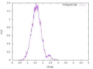
The obtained histogram should look like the following:
- The user should also calculate the mean value and variance of the Cl--Cl- distance. It is recommended to the user to try to write an own script/program doing that. Otherwise the user can calculate the mean by typing "python average_and_standard_deviation.py" on the command line which calls the following python script:
#!/usr/bin/python

import sys
import re
import math

data=[]
readfile = open("timeEvol.dat","r")
line=readfile.readline()
z=0
mean=0.0
standard_deviation=0.0
#loop over lines in file timeEvol.dat
while (line):
  z=z+1
  line.strip()
  line=re.sub('^',' ',line)
  y=line.split()
  #calculate mean
  mean=mean+float(y[0])
  #save data for later
  data.append(float(y[0]))
  line=readfile.readline()
readfile.close
#calculate mean
mean=mean/z
#calculate
for y in data:
   standard_deviation=standard_deviation+(y-mean)**2.0
standard_deviation=(standard_deviation/z)**0.5
print "Mean :",mean
print "Standard devation :",standard_deviation
The calculated mean value and standard deviation should be around 1.49166 and 0.31472 .
Exercise: Did the Cl- ever visit the product's region during this MD?
Higher temperature - 800 K
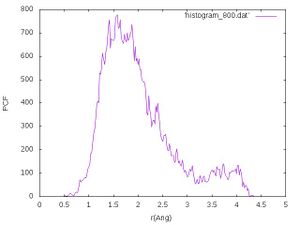
After that we rerun the calculation at 800 K and perform the same analysis steps as above. We should obtain a histogram at 800 K that looks like the following:
The calculated mean value and standard deviation should be around 2.01184 and 0.73784 .
Exercise: Explain the difference at higher temperature!


