Plotting the BSE fatband structure of Si
Task
Visualization of BSE eigenvectors using fatbands.
Input
Si
 5.4300
0.5 0.5 0.0
0.0 0.5 0.5
0.5 0.0 0.5
2
cart
0.00 0.00 0.00
0.25 0.25 0.25
INCAR
- This is the INCAR file for the basic DFT calculation:
System  = Si

PREC = Normal ; ENCUT = 250.0

ISMEAR = 0 ; SIGMA = 0.01
KPAR = 2

EDIFF = 1.E-8
NBANDS = 16
LOPTICS = .TRUE.  # needed for WAVEDER file
LPEAD = .TRUE.
OMEGAMAX = 40
KPOINTS
The KPOINTS file will be automatically generated in this example.
Calculation
- In this example we will calculate and plot the first "bright" BSE eigenstates of silicon, also called fatbands[1]. In this tutorial the modelBSE setup from the previous tutorial is used in combination with a gamma centered k-point grid (if you don't want to wait that long, a grid takes only a minute). In principle the standard BSE method can also be used instead.
Step 1 DFT calculation
We run a standard DFT calculation with the input files given above.
Step 2 BSE calculation with fatbands
- The INCAR file for the modelBSE calculation looks like the following:
System  = Si

PREC = Normal ; ENCUT = 250.0

#ALGO = BSE
ANTIRES = 0
ISMEAR = 0 ; SIGMA = 0.01
ENCUTGW = 150

EDIFF = 1.E-8 # default 1.E-4
NBANDS = 16   # only bands that are used are required, prepare the same set in a forgoing DFT run
NBANDSO = 4
NBANDSV = 8
OMEGAMAX = 20

PRECFOCK = Normal

ALGO = TDHF
LMODELHF = .TRUE. #Turn model on
HFSCREEN = 1.26  # Screening lenght
AEXX = 0.088    #Inverse of epsilon_infinity
SCISSOR = 0.69  # Difference GW-DFT band gap

NBSEEIG = 10 # number of BSE eigenvectors written out in BSEFATBAND
- The important tag for fatband calculations is NBSEEIG. In this example this will write the 10 energetically lowest BSE eigenvectors to the output file BSEFATBAND.
- After the (model)BSE calculation we first look into the vasprun.xml file to have a look at the BSE eigenvalues and the oscillator strengths (exact numbers can of course differ depending on the method you use and the density of your k-point grid):
<varray name="opticaltransitions" >
 <v>      3.148           0.000 </v>
 <v>      3.148           0.000 </v>
 <v>      3.148           0.000 </v>
 <v>      3.149       25654.244 </v>
 <v>      3.149       25660.601 </v>
 <v>      3.149       25665.652 </v>
 <v>      3.151           0.001 </v>
 <v>      3.151           0.001 </v>
 <v>      3.152         423.751 </v>
 <v>      3.310      216931.963 </v>
 <v>      3.310      216916.814 </v>
 <v>      3.310      216935.593 </v>
The first number column shows the BSE eigenvalue and the second one the oscillator strength. We want to plot the first "bright" state, that means in this case number 4.
- We inspect the fourth band in the BSEFATBAND output file:
             28428                10
     1BSE eigenvalue    3.14798542      IP-eigenvalue:    3.25790292
  0.00000  0.00000  0.00000    -6.1302666     9.0994773       0.0000001     1     5     -0.000000+i*    -0.000000
  0.00000  0.00000  0.00000     5.8415744     9.0994773       0.0876503     2     5      0.000076+i*     0.000043
  0.00000  0.00000  0.00000     5.8415744     9.0994773     341.0850802     3     5      0.088630+i*    -0.329369
  0.00000  0.00000  0.00000     5.8415744     9.0994773     543.1678695     4     5      0.361803+i*    -0.405130
  0.00000  0.00000  0.00000    -6.1302666     9.0994773       0.0000004     1     6     -0.000000+i*     0.000000
…(28428-6 more lines till 2BSE eigenvalue …)
     4BSE eigenvalue    3.14855812      IP-eigenvalue:    3.25790292
  0.00000  0.00000  0.00000    -6.1302666     9.0994773       0.0024165     1     5      0.000002+i*     0.000001
  0.00000  0.00000  0.00000     5.8415744     9.0994773      31.4738813     2     5     -0.027821+i*    -0.014718
  0.00000  0.00000  0.0000File:Fig BSE example3 1.png0     5.8415744     9.0994773     187.8684774     3     5      0.049093+i*    -0.181341
  0.00000  0.00000  0.00000     5.8415744     9.0994773     360.1697144     4     5      0.239775+i*    -0.268757
  0.00000  0.00000  0.00000    -6.1302666     9.0994773       0.0289534     1     6      0.000019+i*    -0.000022
...
The description of the values is given as follows:
- line: Number of e-h pairs in the BSE basis and value for NBSEEIG.
- line: BSE eigenvalue and minimum band gap before BSE.
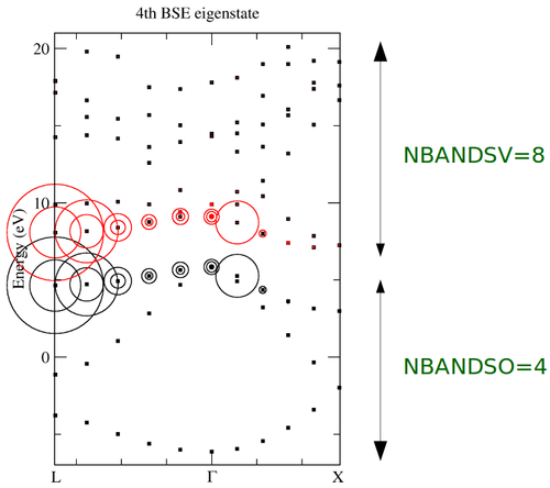
- line: Column 1-3 k-point coordinate, column 4 hole eigenvalue, column 5 electron eigenvalue, column 6 absolute value of coupling coefficient (radius of circles), column 7 hole orbital, column 8 electron number, column 9 real part of coupling coefficient, column 10 imaginary part of coupling coefficient.
Columns 1-6 are used to plot the fatbands.
- Plotting of data:
- Select the BSE eigenstate from the FATBAND file which you want to plot.
- Filter out all e-h pairs that lie on the high symmetry k-lines along which you want to plot the fat bandstructure:
#!/bin/bash

head -n  113716  BSEFATBAND > tmTry: NBANDSO=NBANDSV=2
and check how much this effects the bse results.p.dat
tail -n  28428  BSEFATBAND > BSE4.dat
rm tmp.dat

awk <BSE4.dat  ' { if ($1==$2 && $3==$2) print sqrt($1*$1+$2*$2+$3*$3), $4, $5, $6 }' >bands-GL.dat
awk <BSE4.dat  ' { if ($1==$3 && $2==0.0) print sqrt($1*$1+$2*$2+$3*$3), $4, $5, $6 }' >bands-GX.dat
- Use your favourite tool to plot the output in the following manner:
|k-point|   electron        hole          |A|
           eigenvalue    eigenvalue
    x          y1            y2         radius
File:Fig BSE example3 1.png
- The sample output for this tutorial should look like the following:
The fat band picture allows you to visually inspect which e-h pairs contribute the most to a particular BSE eigenstate. When k-point convergence is important, you can use it to truncate your e-h product basisset by choosing smarter NBANDSO/NBANDSV and/or OMEGAMAX values. Try NBANDSO=NBANDSV=2and check how much this effects the BSE results.
Download
References
Back to the main page

