Improving the dielectric function: Difference between revisions
| Line 40: | Line 40: | ||
* Model-BSE: | * Model-BSE: | ||
:Use a parametrized model<ref name="bokdam:scr:6"/> | :Use a parametrized model<ref name="bokdam:scr:6"/><ref name="liu:bse"/> for the dielectric screening, and DFT eigenenergies moved with a ''scissor'' operator, instead of RPA screening and GW quasiparticle energies. | ||
=== Averaging over multiple grids === | === Averaging over multiple grids === | ||
Revision as of 12:08, 17 September 2019
Task
Calculate the dielectric function of Si using an averaging over multiple grids or a model-BSE to improve k-sampling in BSE calculations.
Input
Si
 5.4300
0.5 0.5 0.0
0.0 0.5 0.5
0.5 0.0 0.5
2
cart
0.00 0.00 0.00
0.25 0.25 0.25
INCAR
- This is the INCAR file for the basic DFT calculation:
System  = Si
PREC = Normal ; ENCUT = 250.0
ISMEAR = 0 ; SIGMA = 0.01
KPAR = 2
EDIFF = 1.E-8
KPOINTS
Automatic
 0
Gamma
 4 4 4
 0 0 0
Calculation
The calculated spectra can be improved in two ways:
- Averaging over multiple grids:
- Compute N independent dielectric functions using BSE (or any other method), using shifted grids of k-points, and take the average over the results.
- Model-BSE:
- Use a parametrized model[1][2] for the dielectric screening, and DFT eigenenergies moved with a scissor operator, instead of RPA screening and GW quasiparticle energies.
Averaging over multiple grids
- Construct shifted k-point grid with the same density.
- k-point grid irreducible k-points with weights . We do calculations on a grid, shifted of Gamma by .
- Extract the dielectric function of each calculation and average over them with respect to the weights :
We have now effectively constructed the result for a grid. But interactions of range longer than times the supercell size have been ignored.
- In our example we use and : Effectively we use k-points.
- In the script doall-average.sh the scheme is written for and . At the end the dielectric functions are extracted and averaged accordingly. You can choose up to which level of theory (DFT, RPA, BSE) the dielectric function is computed by commenting out the corresponding lines in the script (default is all the way up to BSE).
- Because of the shifted grids we have to use density functional perturbation theory to calculate the derivatives of the wave functions with respect to and not the finite difference scheme. We also have to switch off all k-points symmetry in all INCAR files. These two important parameters look like the following in the INCAR file:
PREC = Normal ; ENCUT = 250.0

ALGO = EXACT ; NELM = 1
ISMEAR = 0 ; SIGMA = 0.01
KPAR = 2

NBANDS = 32 # The number of bands in the consecutive BSE calculation should be the same!
LOPTICS = .TRUE.; LPEAD = .FALSE.
ISYM = -1
OMEGAMAX = 40
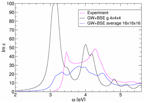
- Finally the averaging over multiple grids should should give spectra that are in much closer agreement than the calculations using k-points:
Model-BSE
The dielectric function is replaced by the local model function:
- .
This makes the screened Coulomb kernel diagonal in the screened Coulomb potential:
- ,
where denote Bloch integrals of the cell-periodic part of the Bloch waves.
- In addition to a model dielectric function we need approximate quasiparticle energies and wave functions.
- Approximation:
- Use DFT single particle eigenvalues + SCISSOR (SCISSOR=GW band gap - DFT band gap).
- Use DFT single particle orbitals.
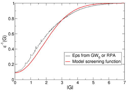
- Extract dielectric function from the vasprun.xml file from the previous GW calculation using the script ./extract_die_G.sh vasprun.xml > dieG_g6x6x6-GW0.dat' or view the attached file dieG_g6x6x6-GW0.dat. Use AEXX=0.088 for and HFSCREEN=1.26 for .Then fit the model to get:
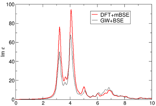
- Check the GW+BSE and DFT+mBSE calculations for constistency:
- The sequence of calculations as given in the script doall-model.sh consists of two steps:
- Step 1: standard DFT calculation. The INCAR file (INCAR.DFT) for this step looks as follows:
PREC = Normal ; ENCUT = 250.0
ISMEAR = 0 ; SIGMA = 0.01
EDIFF = 1.E-8
NBANDS = 16
PRECFOCK = Normal

#WAVEDER file must be made:
LOPTICS = .TRUE.
LPEAD = .TRUE.
OMEGAMAX = 40
- Step2: model BSE calculation. The INCAR file (INCAR.mBSE) for this step looks as follows:
PREC = Normal ; ENCUT = 250.0

ALGO = TDHF
ANTIRES = 0 ; SIGMA = 0.01
ENCUTGW = 150

EDIFF = 1.E-8
NBANDS = 16
NBANDSO = 4
NBANDSV = 8
OMEGAMAX = 20

PRECFOCK = Normal

LMODELHF = .TRUE.
HFSCREEN = 1.26
AEXX = 0.088
SCISSOR = 0.69
- Finally the result of the DFT+mBSE should be of similar accuracy as the GW+BSE calculations when compared to experiment:
Download
References
Back to the main page


