Liquid Si - Freezing: Difference between revisions

Revision as of 12:01, 1 October 2019

Overview >Liquid Si - Standard MD > Liquid Si - Freezing > Nucleophile Substitution CH3Cl - Standard MD > Nuclephile Substitution CH3Cl - mMD1 > Nuclephile Substitution CH3Cl - mMD2 > Nuclephile Substitution CH3Cl - mMD3 > Nuclephile Substitution CH3Cl - SG > Nuclephile Substitution CH3Cl - BM > List of tutorials

Task

In this example the goal is to simulate the freezing of liquid Si.

Input

POSCAR

Si
15.12409564534287297131
     0.5000000000000000    0.5000000000000000    0.0000000000000000
     0.0000000000000000    0.5000000000000000    0.5000000000000000
     0.5000000000000000    0.0000000000000000    0.5000000000000000
  48
Direct
  0.8550657259653851  0.3204575801875221  0.6180363868822553
  0.6045454476433229  0.0546379652195404  0.1629680405553871
  0.4803889256776521  0.2999635319377835  0.0131251454718051
  0.8413504226620471  0.7598095803296524  0.1917781560970181
  0.9754163118144437  0.6134171268457649  0.7421364242876367
  0.2668229391055025  0.0066502741664650  0.0031140604380929
  0.8935777664000575  0.3324172908647429  0.9535738516718881
  0.0527608886321274  0.5249316429131962  0.5293744880144071
  0.4396089233132741  0.7564833235979471  0.5665855438788387
  0.5907859878830199  0.5198033580597228  0.3581725847640679
  0.2120832721474721  0.4042899613004446  0.7921535013319151
  0.0225803885096466  0.8414911198321031  0.1209255489569852
  0.0992500701525566  0.3917384466892963  0.3612433325214984
  0.9673794138223195  0.5206425706394114  0.1719623236201897
  0.2774602656926126  0.8480860088162007  0.2673309412777037
  0.0196991774214161  0.8282178425383616  0.6986213756952502
  0.3570927152895376  0.2951488295546784  0.2651851032568589
  0.1663829731894614  0.9766237917413699  0.6051764245375237
  0.4931841331696695  0.8689890620771937  0.2612357008392290
  0.8006473407426477  0.1033419073227807  0.4706563716777467
  0.0161340851939779  0.9953827418297991  0.8853439845676159
  0.7827740166661069  0.1821830067208054  0.9399555168314748
  0.0720651739141343  0.2539424963694544  0.6857919074323433
  0.4443385370769313  0.0486404637002326  0.4180706114402839
  0.7055263679666055  0.6802623819082319  0.7983614866719116
  0.2237125282521105  0.4055474352416297  0.0077044950891134
  0.2963682069847125  0.5771265542042112  0.2019757061665083
  0.2782449529809642  0.0451513130915826  0.7644934848784113
  0.9312079203181675  0.9090938018377080  0.3429249881187518
  0.6341882597200124  0.2969253226419481  0.3227590981305088
  0.3587691103780569  0.1061057273904179  0.0931868777500710
  0.8710437838676732  0.6541301230631744  0.4261617089364881
  0.6784300588817769  0.3263889355408940  0.5560491395978739
  0.5597052314845080  0.0174390112509929  0.6129003207931863
  0.0595962318875451  0.1019295953521402  0.3340999072062676
  0.7689671766774326  0.1768870209149794  0.1604177484299765
  0.9603661624482890  0.3311649224573259  0.1439224909303592
  0.3792868784787023  0.2806150985211180  0.4921541531665999
  0.8079860889823454  0.9194188799048340  0.9131036494263627
  0.3002081239026374  0.7834053620019006  0.8650323716139056
  0.4704528574512951  0.7221628305989689  0.9746107190983403
  0.2886552568292480  0.5927625600330780  0.4239421203107919
  0.4116743942942291  0.2198943758058664  0.7072597030225044
  0.2104494234814825  0.6457654201409418  0.8275863924787099
  0.6784628197745537  0.7205455185203838  0.1093053357228383
  0.6344130299021448  0.1650970001101275  0.8037018707797643
  0.3965793440603315  0.5364088146415013  0.6064549771969059
  0.6686412136025504  0.7848666926903073  0.5681234351534038

INCAR

SYSTEM =  Si
# electronic degrees                                                            
LREAL = A                      # real space projection
PREC  = Normal                 # chose Low only after tests
EDIFF = 1E-5                   # do not use default (too large drift)
ISMEAR = -1 ; SIGMA = 0.130    # Fermi smearing: 1500 K 0.086 10-3
ALGO = Very Fast               # recommended for MD (fall back ALGO = Fast)
MAXMIX = 40                    # reuse mixer from one MD step to next
ISYM = 0                       # no symmetry                                    
NELMIN = 4                     # minimum 4 steps per time step, avoid breaking after 2 steps
# MD (do little writing to save disc space)
IBRION = 0                     # main molecular dynamics tag
NSW = 400                      # number of MD steps
POTIM = 3                      # time step of MD
NWRITE = 0                     # controls output
NBLOCK = 10                    # after ten steps pair correlation function is written out
LCHARG = .FALSE.               # no charge density written out
LWAVE = .FALSE.                # no wave function coefficients written out
TEBEG = $i                     # starting temperature for MD
TEEND = $i                     # end temperature for MD
# canonic (Nose) MD with XDATCAR updated every 10 steps
MDALGO = 2                     ä switch to select thermostat
SMASS =  3                     # Nose mass
ISIF = 2                       # this tag selects the ensemble in combination with the thermostat

Most of the tags here are very similar to the tags used in the previous example (Liquid Si - Standard MD).
A stepwise cooling will be applied in this example via a script where $i for TEBEG and TEEND will be replaced in each calculation (see below).

KPOINTS

Si-freezing
0 0 0
Gamma
 1 1 1
 0 0 0

A single k-point is sufficient in this example.

Calculation

We will execute the cooling stepwise so several calculations at different temperatures are required in this calculation. The INCAR is created with a script for each temperature and run separately. After each step the important files are saved to file.$i, where $i are the temperatures ranging from 2000 to 800 K in steps of 100 K. The script running the calculations looks like the following:

for i in 2000 1900 1800 1700 1600 1500 1400 1300 1200 1100 1000 900 800
do
cat >INCAR <<!
SYSTEM =  Si
# electronic degrees                                                            
LREAL = A                      # real space projection
PREC  = Normal                 # chose Low only after tests
EDIFF = 1E-5                   # do not use default (too large drift)
ISMEAR = -1 ; SIGMA = 0.130    # Fermi smearing: 1500 K 0.086 10-3
ALGO = Very Fast               # recommended for MD (fall back ALGO = Fast)
MAXMIX = 40                    # reuse mixer from one MD step to next
ISYM = 0                       # no symmetry                                    
NELMIN = 4                     # minimum 4 steps per time step, avoid breaking after 2 steps
# MD (do little writing to save disc space)
IBRION = 0                     # main molecular dynamics tag
NSW = 400                      # number of MD steps
POTIM = 3                      # time step of MD
NWRITE = 0                     # controls output
NBLOCK = 10                    # after ten steps pair correlation function is written out
LCHARG = .FALSE.               # no charge density written out
LWAVE = .FALSE.                # no wave function coefficients written out
TEBEG = $i                     # starting temperature for MD
TEEND = $i                     # end temperature for MD
# canonic (Nose) MD with XDATCAR updated every 10 steps
MDALGO = 2                     ä switch to select thermostat
SMASS =  3                     # Nose mass
ISIF = 2                       # this tag selects the ensemble in combination with the thermostat
!
mpirun -np 2 /path/to/your/vasp/executable
cp XDATCAR XDATCAR.$i
cp OUTCAR OUTCAR.$i
cp PCDAT PCDAT.$i
cp CONTCAR CONTCAR.$i
cp POSCAR POSCAR.$i
cp OSZICAR OSZICAR.$i
cp CONTCAR POSCAR
done

Before running the script one has to replace "'/path/to/your/vasp/executable'" by the path to his "'vasp_gam'" executable. The script is then simply starte by typing the following command in the command line:

bash ./script

Diffusion

The diffusion coefficient in 3 dimensions is given as

$D=\frac{\langle x^{2} \rangle} {6 t}$

where t defines time and $\langle x^{2} \rangle$ . The 6 in the denominator contains a factor of 3 accounting for the 3 spatial dimensions (usually the diffusion coefficient is written with a 2 in the denominator in literature corresponding to only one dimension). In our case we calculate the above equation as follows

$D=\frac{\langle \sum_{i}^{N} [x_{i}(t)-x_{i}(0)]^{2} \rangle}{6 \Delta t}$ .

Here the diffusion coefficient is calculated over an ensemble average to get better statistics. Our calculations were carried out for 1200 fs for each temperature. We will average in our case over the last 900 fs regarding the first 300 fs as equilibration of each temperature. The following python script (diffusion_coefficient.py) calculates the diffusion coefficient at a given temperature:

Click to show/diffusion_coefficient.py

Diffusion coefficient liquid Si freezing

Since the atoms can move such that the distance between old and new position becomes larger than 0.5 (in crystallographic or fractional coordinates). Let us take for example the movement of atom 0 in the $x$ direction from 0 to -0.25, which would be output in the CONTCAR as 0.75. The distance corresponding to that would be than calculated as 0.75 which is wrong since we have periodic images and the real shortest distance would be 0.25. Hence all distance larger than 0.5 have to be shifted by -1.0. This is taken care in the script.

We will use a short bash script (dscript.sh) to calculate the diffusion coefficient at different temperatures and plot them in a file (diff_coeff.jpg):

#!/bin/bash

if test -f "diff_coeff.dat"; then
   rm diff_coeff.dat
fi

touch diff_coeff.dat

for i in 800 900 1000 1100 1200 1300 1400 1500 1600 1700 1800 1900 2000; do
   diffusion_coefficient.py XDATCAR.$i >>  diff_coeff.dat
done

gnuplot -e "set terminal jpeg; set key left; set xlabel 'temperature (K)'; set ylabel 'D (Ang^2/ps)'; set style data lines; plot 'diff_coeff.dat' " > diff_coeff.jpg

To execute it just type the following command:

bash ./dscript.sh

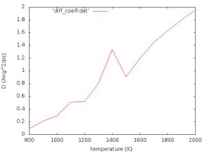
The data for the diffusion coefficient at each temperature is output to diff_coeff.dat and plotted in diff_coeff.jpg which should look like the following:

Exercise: Interpret Fig. 1 yourself!

Solution: For a given phase the diffusion coefficient depends directly on the temperature by

$D=\mu k_{B} T$

where $k_{B}$ is the Boltzmann constant and $\mu$ is the mobility of the particle. Evidently this relation is approximately fulfilled in Fig. 1. At approximately 1400 K we see a peak. This temperature should correspond to the phase transition temperature. Close to the phase transition point the scaling with respect to the reduced temperature $T_{\mathrm{red}}$ becomes

$\langle x^{2} \rangle \propto T_{\mathrm{red}}^{1-\alpha},\qquad \qquad \qquad T_{\mathrm{red}}=\frac{T-T_{c}}{T_{c}}$

where $\alpha$ is an anomalous dimension (it may be positive or negative) and $T_{c}$ is the critical temperature. For infinite large systems and infinite time this would lead to a singularity in the plot, but since we are dealing with a finite sized system it results in a finite peak at the phase transition point.

Pair correlation function

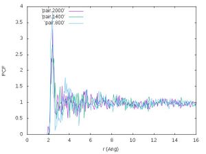
The pair-correlation function provides information about the probability of finding two atoms at a given distance $r$ . The pair-correlation function is save for each temperature under PCDAT.T. The following script will plot the pair correlation functions at different temperatures in one figure:

#!/bin/bash

for i in 800 900 1000 1100 1200 1300 1400 1500 1600 1700 1800 1900 2000; do
   awk <PCDAT.$i >pair.$i ' NR==8 {pcskal=$1} NR==9 {pcfein=$1} NR>=10036 {line=line+1; print (line-0.5)*pcfein/pcskal,$1} '
done

gnuplot -e "set terminal jpeg; set key left; set xlabel 'r (Ang)'; set ylabel 'PCF'; set style data lines; plot 'pair.2000','pair.1400','pair.800' " > pair.jpg

To execute it type the following command:

bash ./pair.sh

The plot should look like the following:

User task: Interpret the figure yourself!

Solution: Crystalline structures usually have less diffuse pair correlation functions since the atoms are usually vibrating around high symmetry points. In liquids the average positions are smeared out over a wider range of distances. With decreasing temperature the pair correlation function in the plot gets more structured. This indicates that crystallization is happening.

Download

Si_Liquid_Freezing.tgz

Overview > fcc Si > fcc Si DOS > fcc Si bandstructure > cd Si > cd Si volume relaxation > cd Si relaxation > beta-tin Si > fcc Ni > graphite TS binding energy > graphite MBD binding energy > graphite interlayer distance > List of tutorials

Revision as of 11:53, 1 October 2019 (view source) Karsai (talk \| contribs) (→‎Diffusion) ← Older edit		Revision as of 12:01, 1 October 2019 (view source) Karsai (talk \| contribs) No edit summary Newer edit →
Line 182:		Line 182:
	[[File:Diff coeff.jpg\|300px\|]]		[[File:Diff coeff.jpg\|300px\|]]

	'''~~User task~~''': Interpret Fig. 1 yourself!		'''Exercise''': Interpret Fig. 1 yourself!