Part 1: Melting silicon 
By the end of this tutorial, you will be able to:
- state what ab-initio molecular dynamics (MD) refers to
- create supercells and handle the Crystallographic Information File (CIF) format using pymatgen
- tell the difference between vasp_gam and vasp_std
- distinguish and plot different energies in the context of MD calculations over time steps using py4vasp
- plot MD trajectories using py4vasp
1.1 Task
Perform an ab-initio MD simulation for cubic-diamond (cd) silicon for 90fs with 64 atoms in a canonical ensemble using the Nosé-Hoover thermostat at 2000 K.
In MD simulations, the motion of atoms (or molecules) at a specific temperature is simulated by means of the classical equation of motion. In other words, each iteration simulates a time step, where atoms are treated as classical particles subject to forces as in Newton's second law. When these forces are computed quantum mechanically using ab-initio methods, one speaks of ab-initio MD. To employ the canonical ensemble, or NVT ensemble, the calculation must be done at constant number of particles (N), constant volume (V) and constant temperature (T).
To include the effect of temperature, some kind of thermostat needs to be included. Methods to achieve that involve modifying the equations of motion either by introducing stochastic or deterministic terms through additional dynamical variables, which mimic the action of a heat bath in a real thermostat. The Nosé-Hoover thermostat corresponds to the latter. A possible deficiency of the Nosé-Hoover thermostat is the lack of ergodicity in small or stiff systems, for instance in the simulation of a single butane molecule, but it is perfectly suitable for the present example.
In order to learn more about MD algorithms in VASP and how the effect of temperature is included by means of the Nosé-Hoover thermostat in this calculation, read the linked VASP Wiki articles.
1.2 Input
The input files to run this example are prepared at $TUTORIALS/MD/e01_solid-cd-Si.
The conventional unit cell for the cd silicon structure is provided as a Crystallographic Information File (CIF). CIFs are the standard for crystallographic data exchange prescribed by the International Union of Crystallography. To create a POSCAR file based on a CIF you can use the Python Materials Genomics (pymatgen) package, which is an open-source Python library for materials analysis. Many MD calculations are done with a supercell spanning multiple conventional unit cells. This is, to capture all lattice vibrations that affect the essential dynamics of the system. In practice, it is expedient to carefully check the convergence of the quantity of interest with respect to the cell size.
In pymatgen, you can easily read CIFs, create supercells, and write the appropriate POSCAR file as you can see in the code cell below. Execute the code!
from pymatgen.core import Structure

my_struc = Structure.from_file("./e01_solid-cd-Si/Si_mp-149_conventional_standard.cif")

# make a 2x2x2 supercell
my_struc.make_supercell(2)

# write supercell to POSCAR format with specified filename
my_struc.to(fmt="poscar", filename="./e01_solid-cd-Si/POSCAR")

# A POSCAR file will appear at $TUTORIALS/MD/e01_solid-cd-Si
# You may need to refresh the file browser to see it
Why do we use a supercell to perform MD simulations?
Click to see the answer!
The size of the supercell imposes a limit on the maximum wavelength of lattice vibrations. The supercell used in an MD simulation should be large enough to account for all vibration modes with significant contribution to the specific quantity of interest to be computed in MD. This can be estimated, e.g., from an appropriate phonon calculation, or from a series of MD simulations with different supercell sizes.
Furthermore, in calculations considering for instance an adsorbate-substrate problem, or simulations of gases and liquids, the size of the unit cell should be large enough to remove unphysical interactions between atoms and their periodic images. Note that, the same holds also for relaxations of such systems.
In summary, for your MD simulation, you should choose a supercell large enough to ensure an ergodic simulation and capture all long-wavelength vibrations of your system.
Click to see POSCAR file generated from CIF!
Si64
1.0
10.937456 0.000000 0.000000
0.000000 10.937456 0.000000
0.000000 0.000000 10.937456
Si
64
direct
0.125000 0.375000 0.125000 Si
0.125000 0.375000 0.625000 Si
0.125000 0.875000 0.125000 Si
0.125000 0.875000 0.625000 Si
0.625000 0.375000 0.125000 Si
0.625000 0.375000 0.625000 Si
0.625000 0.875000 0.125000 Si
0.625000 0.875000 0.625000 Si
0.000000 0.000000 0.250000 Si
0.000000 0.000000 0.750000 Si
1.000000 0.500000 0.250000 Si
1.000000 0.500000 0.750000 Si
0.500000 0.000000 0.250000 Si
0.500000 0.000000 0.750000 Si
0.500000 0.500000 0.250000 Si
0.500000 0.500000 0.750000 Si
0.125000 0.125000 0.375000 Si
0.125000 0.125000 0.875000 Si
0.125000 0.625000 0.375000 Si
0.125000 0.625000 0.875000 Si
0.625000 0.125000 0.375000 Si
0.625000 0.125000 0.875000 Si
0.625000 0.625000 0.375000 Si
0.625000 0.625000 0.875000 Si
1.000000 0.250000 0.000000 Si
1.000000 0.250000 0.500000 Si
1.000000 0.750000 0.000000 Si
1.000000 0.750000 0.500000 Si
0.500000 0.250000 0.000000 Si
0.500000 0.250000 0.500000 Si
0.500000 0.750000 1.000000 Si
0.500000 0.750000 0.500000 Si
0.375000 0.375000 0.375000 Si
0.375000 0.375000 0.875000 Si
0.375000 0.875000 0.375000 Si
0.375000 0.875000 0.875000 Si
0.875000 0.375000 0.375000 Si
0.875000 0.375000 0.875000 Si
0.875000 0.875000 0.375000 Si
0.875000 0.875000 0.875000 Si
0.250000 0.000000 0.000000 Si
0.250000 0.000000 0.500000 Si
0.250000 0.500000 0.000000 Si
0.250000 0.500000 0.500000 Si
0.750000 0.000000 0.000000 Si
0.750000 0.000000 0.500000 Si
0.750000 0.500000 1.000000 Si
0.750000 0.500000 0.500000 Si
0.375000 0.125000 0.125000 Si
0.375000 0.125000 0.625000 Si
0.375000 0.625000 0.125000 Si
0.375000 0.625000 0.625000 Si
0.875000 0.125000 0.125000 Si
0.875000 0.125000 0.625000 Si
0.875000 0.625000 0.125000 Si
0.875000 0.625000 0.625000 Si
0.250000 0.250000 0.250000 Si
0.250000 0.250000 0.750000 Si
0.250000 0.750000 0.250000 Si
0.250000 0.750000 0.750000 Si
0.750000 0.250000 0.250000 Si
0.750000 0.250000 0.750000 Si
0.750000 0.750000 0.250000 Si
0.750000 0.750000 0.750000 Si
SYSTEM = cd Si

! ab initio
ISMEAR = 0        ! Gaussian smearing
SIGMA  = 0.1      ! smearing in eV

LREAL  = Auto     ! projection operators in real space

ALGO   = VeryFast ! RMM-DIIS for electronic relaxation
PREC   = Low      ! precision
ISYM   = 0        ! no symmetry imposed

! MD
IBRION = 0        ! MD (treat ionic degrees of freedom)
NSW    = 30       ! no of ionic steps
POTIM  = 3.0      ! MD time step in fs

MDALGO = 2        ! Nosé-Hoover thermostat
SMASS  = 1.0      ! Nosé mass

TEBEG  = 2000     ! temperature at beginning
TEEND  = 2000     ! temperature at end
ISIF   = 2        ! update positions; cell shape and volume fixed
Gamma-point only
 0
Monkhorst Pack
 1 1 1
 0 0 0
Pseudopotentials of Si.
Check the tags set in the INCAR file!
The first six tags, ISMEAR, SIGMA, LREAL, ALGO, PREC and ISYM, concern the computation of the Kohn–Sham (KS) orbitals.
The remaining tags specify the settings for the MD simulation. IBRION = 0 switches on MD. Then, NSW and POTIM set the number of ionic updates and the step size. For MD, the step size is a unit of time given in fs.
MDALGO sets the thermostat. We use the Nosé-Hoover thermostat, where the flow of energy between the physical system and the heat reservoir is regulated by the thermal inertia, or Nosé mass, SMASS. To realize an NVT ensemble, the temperature at the beginning and at the end, i.e., TEBEG and TEEND, are equal and the volume is kept fixed with ISIF = 2.
The KPOINTS file specifies a single $\mathbf{k}$ point: The so-called Γ point at $\mathbf{k}=(0,0,0)$. This is enough, because you are using a large supercell.
1.3 Calculation
Open a terminal, navigate to this example's directory and run VASP by entering the following:
cd $TUTORIALS/MD/e01_*
mpirun -np 2 vasp_gam
This calculation is done using vasp_gam, which got its name from the fact that it can only perform calculations at the Γ point. Underneath that implies that the KS orbitals can be considered to be real valued. That means if you run the same calculation with vasp_gam and vasp_std, vasp_gam is faster.
Let us have a closer look at the standard output (stdout), that is printed to the terminal during the calculation. Note that every run is different because it starts from a different random seed.
Click to see the stdout!
 running on    2 total cores
 distrk:  each k-point on    2 cores,    1 groups
 distr:  one band on    1 cores,    2 groups
 vasp.6.3.0 16May21 (build Oct 27 2021 15:52:58) gamma-only

 POSCAR found type information on POSCAR Si
 POSCAR found :  1 types and      64 ions
 Reading from existing POTCAR
 scaLAPACK will be used
 Reading from existing POTCAR
 LDA part: xc-table for Pade appr. of Perdew
 POSCAR, INCAR and KPOINTS ok, starting setup
 FFT: planning ...
 WAVECAR not read
 prediction of wavefunctions initialized - no I/O
 entering main loop
       N       E                     dE             d eps       ncg     rms          rms(c)
RMM:   1     0.155222068701E+04    0.15522E+04   -0.44526E+04   162   0.508E+02
RMM:   2     0.297589951477E+03   -0.12546E+04   -0.12725E+04   162   0.145E+02
RMM:   3    -0.664488972878E+02   -0.36404E+03   -0.43415E+03   162   0.787E+01
RMM:   4    -0.220663864053E+03   -0.15421E+03   -0.16002E+03   162   0.560E+01
RMM:   5    -0.287411476155E+03   -0.66748E+02   -0.65206E+02   162   0.316E+01
RMM:   6    -0.320343488885E+03   -0.32932E+02   -0.28274E+02   162   0.212E+01
RMM:   7    -0.334632556790E+03   -0.14289E+02   -0.12331E+02   162   0.124E+01
RMM:   8    -0.340563651457E+03   -0.59311E+01   -0.53511E+01   162   0.792E+00
RMM:   9    -0.344491928264E+03   -0.39283E+01   -0.38231E+01   349   0.472E+00
RMM:  10    -0.344908101129E+03   -0.41617E+00   -0.41412E+00   352   0.165E+00
RMM:  11    -0.344951509187E+03   -0.43408E-01   -0.32463E-01   344   0.581E-01
RMM:  12    -0.344962136179E+03   -0.10627E-01   -0.10202E-01   336   0.281E-01    0.358E+01
RMM:  13    -0.340710112381E+03    0.42520E+01   -0.23514E+00   417   0.230E+00    0.221E+01
RMM:  14    -0.338768179258E+03    0.19419E+01   -0.54002E+00   463   0.369E+00    0.108E+00
RMM:  15    -0.338786847044E+03   -0.18668E-01   -0.10702E-01   324   0.600E-01    0.444E-01
RMM:  16    -0.338800009272E+03   -0.13162E-01   -0.16991E-02   327   0.294E-01    0.381E-01
RMM:  17    -0.338801421308E+03   -0.14120E-02   -0.26217E-03   321   0.108E-01    0.696E-02
RMM:  18    -0.338801478964E+03   -0.57656E-04   -0.60546E-04   262   0.494E-02
    1 T=  2000. E= -.32251463E+03 F= -.33880148E+03 E0= -.33880148E+03  EK= 0.16287E+02 SP= 0.00E+00 SK= 0.00E+00
 bond charge predicted
       N       E                     dE             d eps       ncg     rms          rms(c)
RMM:   1    -0.337852804095E+03    0.94862E+00   -0.22457E+01   324   0.780E+00    0.189E+00
RMM:   2    -0.338087873331E+03   -0.23507E+00   -0.24923E+00   325   0.306E+00    0.108E+00
RMM:   3    -0.338132790582E+03   -0.44917E-01   -0.50218E-01   340   0.124E+00    0.110E+00
RMM:   4    -0.338121036810E+03    0.11754E-01   -0.79021E-02   324   0.547E-01    0.579E-01
RMM:   5    -0.338129671306E+03   -0.86345E-02   -0.76437E-02   324   0.388E-01    0.314E-01
RMM:   6    -0.338123062866E+03    0.66084E-02   -0.16448E-02   326   0.207E-01    0.114E-01
RMM:   7    -0.338122886896E+03    0.17597E-03   -0.90935E-03   323   0.119E-01    0.334E-02
RMM:   8    -0.338122942074E+03   -0.55178E-04   -0.10506E-03   316   0.619E-02    0.244E-02
RMM:   9    -0.338122995490E+03   -0.53416E-04   -0.72833E-04   288   0.348E-02
    2 T=  1916. E= -.32252355E+03 F= -.33812300E+03 E0= -.33812299E+03  EK= 0.15599E+02 SP= -.49E-06 SK= 0.61E-12
 bond charge predicted
 prediction of wavefunctions
       N       E                     dE             d eps       ncg     rms          rms(c)
RMM:   1    -0.336180152440E+03    0.19428E+01   -0.58207E-01   324   0.139E+00    0.654E-01
RMM:   2    -0.336188071907E+03   -0.79195E-02   -0.84588E-02   339   0.505E-01    0.141E-01
RMM:   3    -0.336189675117E+03   -0.16032E-02   -0.16716E-02   353   0.208E-01    0.133E-01
RMM:   4    -0.336189894771E+03   -0.21965E-03   -0.26384E-03   332   0.918E-02    0.929E-02
RMM:   5    -0.336189974660E+03   -0.79889E-04   -0.63462E-04   285   0.448E-02
    3 T=  1685. E= -.32249392E+03 F= -.33618997E+03 E0= -.33618915E+03  EK= 0.13725E+02 SP= -.32E-01 SK= 0.27E-02
 bond charge predicted
 prediction of wavefunctions
       N       E                     dE             d eps       ncg     rms          rms(c)
RMM:   1    -0.333466462434E+03    0.27234E+01   -0.11737E+00   324   0.186E+00    0.677E-01
RMM:   2    -0.333487410180E+03   -0.20948E-01   -0.21196E-01   349   0.731E-01    0.231E-01
RMM:   3    -0.333490239144E+03   -0.28290E-02   -0.30702E-02   343   0.293E-01    0.176E-01
RMM:   4    -0.333490732641E+03   -0.49350E-03   -0.60607E-03   341   0.135E-01    0.933E-02
RMM:   5    -0.333490872875E+03   -0.14023E-03   -0.13599E-03   307   0.636E-02    0.379E-02
RMM:   6    -0.333490903027E+03   -0.30152E-04   -0.32459E-04   233   0.298E-02
    4 T=  1373. E= -.32245824E+03 F= -.33349090E+03 E0= -.33348022E+03  EK= 0.11179E+02 SP= -.18E+00 SK= 0.37E-01
    ...
    ...
    ...
   28 T=  2564. E= -.32254692E+03 F= -.30541712E+03 E0= -.30535338E+03  EK= 0.20878E+02 SP= -.38E+02 SK= 0.13E+00
 bond charge predicted
 prediction of wavefunctions
       N       E                     dE             d eps       ncg     rms          rms(c)
RMM:   1    -0.304962686456E+03    0.45437E+00   -0.50291E-01   338   0.931E-01    0.244E-01
RMM:   2    -0.304975571260E+03   -0.12885E-01   -0.13325E-01   371   0.442E-01    0.982E-02
RMM:   3    -0.304977016808E+03   -0.14455E-02   -0.15036E-02   370   0.179E-01    0.880E-02
RMM:   4    -0.304977314818E+03   -0.29801E-03   -0.32635E-03   345   0.764E-02    0.645E-02
RMM:   5    -0.304977364930E+03   -0.50112E-04   -0.63532E-04   268   0.359E-02
   29 T=  2426. E= -.32253591E+03 F= -.30497736E+03 E0= -.30491565E+03  EK= 0.19755E+02 SP= -.38E+02 SK= 0.28E+00
 bond charge predicted
 prediction of wavefunctions
       N       E                     dE             d eps       ncg     rms          rms(c)
RMM:   1    -0.304475187728E+03    0.50213E+00   -0.47067E-01   340   0.882E-01    0.228E-01
RMM:   2    -0.304487073861E+03   -0.11886E-01   -0.12380E-01   370   0.429E-01    0.918E-02
RMM:   3    -0.304488454010E+03   -0.13801E-02   -0.14617E-02   368   0.176E-01    0.790E-02
RMM:   4    -0.304488726979E+03   -0.27297E-03   -0.30125E-03   343   0.756E-02    0.581E-02
RMM:   5    -0.304488773682E+03   -0.46703E-04   -0.56686E-04   269   0.352E-02
   30 T=  2262. E= -.32252795E+03 F= -.30448877E+03 E0= -.30442641E+03  EK= 0.18424E+02 SP= -.37E+02 SK= 0.41E+00
Information: wavefunction orthogonal band  154  0.8863
 bond charge predicted
 prediction of wavefunctions
 wavefunctions rotated
 writing wavefunctions
After each electronic relaxation, the final line summarizes:
| tag | meaning |
|---|---|
T |
The instantaneous temperature. |
E |
The total energy E including the potential energy F of the ionic degree of freedom, the potential energy SP and kinetic energy SK of the Nose Hoover thermostat, and the kinetic energy of the ionic motion EK. It is called ETOTAL in the OUTCAR file. |
F |
The total free energy of the DFT calculation considering the artificial electronic temperature introduced by the smearing factor SIGMA. In fact, from the view point of MD, this is the potential energy of the ionic degree of freedom. It is called TOTEN in the OUTCAR file. |
E0 |
The total energy of the DFT calculation obtained by subtracting the entropy term and letting SIGMA go to zero for the DFT total free energy F. |
EK |
The kinetic energy of the ionic motion, called EKIN in the OUTCAR file.. |
SP |
The potential energy of the Nosé-Hoover thermostat, called ES in the OUTCAR file. |
SK |
The kinetic energy of the Nosé-Hoover thermostat, called EPS in the OUTCAR file. |
Why is the temperature not constant in every step?
Click to see the answer!
That is the instantaneous temperature and not the observable ensemble average. Note that the idea of a constant temperature calculation is not that the instantaneous temperature is constant in every time step, but that the observable temperature, i.e., the ensemble average of the temperature is constant. You can find the value of the mean temperature <T/S>/<1/S> in the OUTCAR file. In the thermodynamic limit, for sufficiently large number of atoms the fluctuations of the instantaneous temperature would also vanish.
Plot the energies at each time step using py4vasp! Click the label in the legend to interactively select which graph is shown.
import py4vasp
mycalc = py4vasp.Calculation.from_path( "./e01_solid-cd-Si" )
mycalc.energy[:].plot( "TOTEN, ETOTAL" )
mycalc.energy[:].plot( "EKIN, temperature" )
mycalc.energy[:].plot( "ES,EP" )
mycalc.energy[1:5].read()
mycalc.energy[-1].read()
You can now watch how cubic-diamond silicon melts according to your simulation, when it is exposed to 2000 K for 90 fs. Recall that you obtained the forces quantum mechanically from first principles and treated the particles' trajectories classically.
import py4vasp
mycalc = py4vasp.Calculation.from_path( "./e01_solid-cd-Si" )

mycalc.structure[:].plot()
1.4 Questions
- Are trajectories in ab-initio molecular dynamics the paths of quantum mechanical particles?
- What is the standard format to store crystal structure information?
- For what calculations can you use
vasp_gam? - Is the total energy in an NVT ensemble conserved?
- Why do you use large supercells in simulations of molecular dynamics?
By the end of this tutorial, you will be able to:
- compute and interpret the pair-correlation function
- restart an MD simulation
- specify the time of an MD calculation
- find MD trajectories in the XDATCAR file
- set MAXMIX to reduce computational cost
2.1 Task
Compute the pair-correlation function of melting silicon after 90fs, 180fs and 195fs by means of an ab-initio MD simulation for cubic-diamond (cd) silicon with 64 atoms in a canonical ensemble using the Nosé-Hoover thermostat at 2000K.
The structure of a liquid can be studied using the radial distribution function, also known as pair-correlation function. Roughly speaking, it is the probability of finding a particle at a given distance from the center of another particle. More precisely, it is the relative local particle density with respect to the average density of the system at a distance $r$ from the center of an arbitrarily chosen reference particle. Formally, this can be written as $$\tag{2.1} g(r) = \frac{\Omega_r}{N^2} \left\langle \sum_i \sum_{j\neq i} \delta( \mathbf{r} - \mathbf{R}_{ij} ) \right\rangle, $$ where $\Omega_r$ is the real space volume, $N$ is the number of particles, $\mathbf{R}_{ij}= \mathbf{R}_i - \mathbf{R}_{j}$, and $\langle \cdot \rangle$ takes the ensemble average: $$\tag{2.2} \mathcal{A}_{\mathrm{obs}} = \left\langle \mathcal{A}\left(p(t), q(t)\right)\right\rangle_{\mathrm{time}} = \lim_{t_{\mathrm{obs}} \to \infty} \frac{1}{t_{\mathrm{obs}}} \int_0^{t_{\mathrm{obs}}} \, \mathcal{A}\left(p(t), q(t)\right) \, \mathrm{d}t. $$ Here, $\mathcal{A}_{\mathrm{obs}}$ is the observable, macroscopic property, which is written as a time average over $\mathcal{A}\left(p(t), q(t)\right)$ with $p(t)$ and $q(t)$ being the canonical momenta and positions that define the point in phase space that changes over time $t$.
Recall that, in a crystal, we observe long-range order, which leads to distinct peaks in the pair-correlation function. In a liquid state, particles are bound firmly, unlike in gases, but not rigidly, in contrast to solids. The characteristic features of the pair-correlation function change significantly, when a system melts.
What's more, you can use the pair-correlation function to compute the ensemble average of any pair function $\mathcal{B}$ with $$\tag{2.3} \mathcal{B}_{\mathrm{obs}} = \left\langle \sum_i \sum_{j>i} b(\mathbf{R}_{ij}) \right\rangle = \frac{1}{2}N\rho \int_0^\infty b(r)g(r) 4\pi r^2 \mathrm{d}r. $$ This is true for an isotropic liquid, where $\rho$ is the particle density. Read more in Chapter 2.6 of Computer Simulation of Liquids by M. P. Allen and D. J. Tildesley.
2.2 Input
The input files to run this example are prepared at $TUTORIALS/MD/e02_melting-Si.
This calculation is a continuation of Example 1 and requires restarting the MD calculation. That means, you need to copy the latest ionic positions stored in the CONTCAR file of Example 1 to this example's POSCAR file!
Click to see the answer!
cp $TUTORIALS/MD/e01_*/CONTCAR $TUTORIALS/MD/e02_*/POSCAR
Click to see CONTCAR file of Example 1!
Si64
   1.00000000000000
    10.9374559999999992    0.0000000000000000    0.0000000000000000
     0.0000000000000000   10.9374559999999992    0.0000000000000000
     0.0000000000000000    0.0000000000000000   10.9374559999999992
   Si
    64
Direct
  0.0884122650046490  0.3270156326378417  0.1736505382421814
  0.1566955200084217  0.3453583556191027  0.6420065089492452
  0.1227629896024095  0.9068717021822091  0.0972648779388043
  0.1226522769988106  0.8809007833479529  0.6334238722266959
  0.6200180636946139  0.4987085526372492  0.2338488832010892
  0.6539055821210428  0.3272589899341243  0.6573527567755891
  0.6447321012971774  0.8157265736846083  0.1377718241666075
  0.6444283772414973  0.8744777510061614  0.5792440197963021
 -0.0235876162447640  0.0386031146554957  0.1895103955087199
 -0.0183342351026881  0.0269241950809618  0.7388083439310483
  0.0147219235714441  0.4825105694933961  0.2926923259281320
  0.1093376849492344  0.4738036659936390  0.8022133165076762
  0.5074990470988155 -0.0620207772881743  0.2855033790222842
  0.5584989872135804  0.0007453892802960  0.7048520589987353
  0.4395704515759853  0.6063068778853835  0.2833985848402235
  0.4976312784669857  0.4345726225839910  0.7980544611972108
  0.1170700603508791  0.1270538742329672  0.3131555468312924
  0.0301970902882856  0.0933198759716129  0.9412273596919416
  0.0698290663876445  0.5681210369460886  0.4873416699379345
  0.1517645583676528  0.6560064695803963  0.9204828845091002
  0.5624085031256348  0.0981199076767443  0.3986532035242257
  0.6784149503489000  0.1461999050545272  0.8056931722187879
  0.7402114672298926  0.6948673193175292  0.4327068986851282
  0.6299954827461594  0.5630078313839217  1.0146245261114608
 -0.0488385741591179  0.2694313380845236  0.0375669016218063
  0.0442981621268978  0.2886372778708284  0.4461744699190917
 -0.0469946886038712  0.7886141013397897 -0.0475906637161327
 -0.0164988265371824  0.7823022615766945  0.4595347339268085
  0.4711195090180312  0.1244120850803758 -0.1016693628167118
  0.5267247942669063  0.2608499718697633  0.5203979310305102
  0.4649548099513962  0.7800546683219931  0.0194770972357676
  0.4725665493745787  0.7518536573024137  0.4857810594363217
  0.3951071492311899  0.3985542688242734  0.3938602420784584
  0.3275675177401016  0.3002815180159262  0.8568308222716502
  0.3035621684264630  0.8153431672915107  0.2671070196517354
  0.3861506604799382  0.9403307495857870  0.8305747659747484
  0.8121505059008525  0.4216629108673181  0.3334871696711779
  0.9314757442472759  0.4047954878242046  0.8862554137303624
  0.8645557860644485  0.8860062774686731  0.2913354184628085
  0.8342204942300399  0.9063938976985898  0.8271065871715196
  0.2548237220731238  0.0391600243150153 -0.0060011318664706
  0.2235737066721568  0.0066005966574847  0.4657669395191673
  0.2722511038213415  0.4147056956007804  0.0325457156173324
  0.2712576316047652  0.5122368811307643  0.5785155076387282
  0.7660238084286368 -0.0072039504860320  0.0489697480040874
  0.7584869555452394  0.0360539876992204  0.4229322374365250
  0.8375881726407171  0.6079252485169471 -0.1074371119811564
  0.7924651676959711  0.4884830799265052  0.5186721365597021
  0.4792109414605423  0.1310906711412538  0.1834862713412938
  0.3598332092864311  0.1135073263571699  0.5740345067243094
  0.2928107486322241  0.6573562469094013  0.1173597239710458
  0.4114691396046672  0.6025614042017248  0.6899698334261943
  0.7465101295534231  0.2267712976331043  0.0840188387278060
  0.9454397515148174  0.1400400398836375  0.5718084789837456
  0.9281733937705655  0.6260739121117168  0.1211954494269185
  0.9327118205605377  0.5862231886723370  0.6783304739690439
  0.3111233433311294  0.2294601322483154  0.2864947327534821
  0.1770109958804429  0.1287629169606697  0.6788151315712396
  0.1203503741121596  0.7497837593131993  0.2325552175770395
  0.2760906956355750  0.7644377647148360  0.7823799400297161
  0.5968910477128486  0.2711100965081311  0.2601059207196711
  0.8827962514248557  0.2428896087846563  0.7539033351062576
  0.7594060565300381  0.6678693616502112  0.2348027384012320
  0.7627441944075757  0.7201168516282580  0.7270643519527493

 -0.15299595E-01  0.42048068E-02  0.11217434E-01
  0.16365637E-01 -0.76587253E-02  0.40533645E-02
  0.10045262E-01  0.73051058E-02 -0.17877328E-01
  0.35942103E-03 -0.48788581E-02  0.89165170E-02
 -0.11574220E-01 -0.72579935E-03  0.12315747E-01
  0.34231318E-02  0.14167828E-02 -0.47120095E-03
  0.10211030E-01 -0.45159095E-02  0.61744975E-02
  0.26864481E-02  0.69078849E-02 -0.18399792E-02
 -0.45784219E-02  0.12759007E-01 -0.12344851E-01
 -0.33057947E-02 -0.22459821E-02  0.43493558E-02
 -0.27007592E-02 -0.12976110E-02 -0.15705000E-02
  0.55447770E-02  0.17338743E-01 -0.48971740E-02
  0.20128144E-02 -0.41784364E-02  0.13674236E-02
  0.22434547E-02 -0.11990990E-01 -0.81890840E-03
 -0.11357118E-01  0.19117646E-01 -0.88534876E-03
 -0.50418822E-02  0.36069983E-02 -0.82292635E-03
 -0.47010096E-02  0.12655221E-02 -0.13798825E-01
 -0.81972775E-02  0.16853994E-02 -0.35364542E-02
 -0.78112545E-02 -0.98104743E-02 -0.47470834E-02
  0.88555563E-02  0.58198839E-02  0.37171254E-02
  0.95772505E-02  0.59284079E-02  0.43170451E-02
 -0.35179342E-02  0.32209236E-02 -0.13938768E-01
  0.12257604E-01  0.80053612E-02 -0.85974576E-02
  0.11013121E-01 -0.38280804E-02 -0.18080010E-02
  0.76345275E-03 -0.10795724E-01 -0.17427235E-02
  0.55501741E-02 -0.60800542E-02  0.25640582E-02
  0.39378821E-02 -0.27608331E-02 -0.50721752E-02
 -0.72089067E-02 -0.26440723E-02 -0.59197119E-02
 -0.21247157E-02 -0.97571398E-02 -0.72841293E-02
 -0.20064985E-02 -0.97048916E-02  0.30140612E-02
 -0.62319237E-02 -0.84700648E-02  0.64235117E-02
  0.75145043E-04 -0.23738590E-01 -0.32187420E-02
  0.52958905E-02  0.15961919E-01  0.26872630E-02
 -0.60204797E-02  0.18711138E-02  0.33591033E-02
  0.10935892E-01  0.86807154E-03  0.12744997E-02
 -0.64734640E-02 -0.10483558E-01  0.21914256E-02
  0.15074124E-03  0.50803609E-02  0.10885706E-01
 -0.53497134E-03  0.11840858E-04  0.11748716E-01
  0.59306845E-02  0.93697421E-02  0.78165557E-02
  0.24115366E-02  0.12096671E-01 -0.10152273E-03
 -0.86724323E-02  0.41833173E-02 -0.70693175E-02
 -0.10167947E-02  0.14902881E-01  0.36955302E-02
  0.12723483E-01 -0.66252980E-02  0.71215087E-02
  0.68297963E-02  0.91606288E-04  0.58139328E-02
  0.67223546E-02  0.18373147E-02  0.13972346E-01
  0.31864806E-02 -0.10834842E-01  0.74747067E-02
 -0.99506355E-02 -0.21756313E-02 -0.12947958E-01
  0.18903884E-02 -0.76627419E-02 -0.74760613E-02
 -0.44901442E-02 -0.27164187E-02  0.53257563E-02
 -0.48808776E-03  0.57717771E-02 -0.90648203E-02
 -0.79177062E-02 -0.58417988E-02 -0.36075581E-02
 -0.10456922E-01  0.90867352E-02  0.48886394E-02
  0.18902772E-03 -0.61079259E-02 -0.43050853E-02
 -0.17612421E-01 -0.41441803E-02  0.73177163E-02
 -0.18044653E-01  0.50883874E-02 -0.98722238E-02
  0.25669670E-02 -0.15070077E-01  0.44239101E-02
  0.10008193E-01  0.89651187E-02  0.26698226E-02
  0.57692280E-02 -0.15191451E-01 -0.31532964E-02
 -0.54356189E-02 -0.19777113E-02  0.74857851E-02
  0.13737605E-01 -0.12513260E-01 -0.11736082E-01
 -0.14815418E-01  0.14276008E-01  0.43639841E-02
 -0.13330854E-02  0.40938387E-02  0.35467776E-03
  0.75109728E-02 -0.14490002E-02  0.59213873E-02
  0.81387428E-02  0.15736955E-01 -0.86968997E-02

           1
   3.00000000000000
 -0.12246449E+01 -0.31444762E-01 -0.33928700E-01 -0.11919582E+01
  0.84215788E-01  0.32816896E+00  0.17672733E+00
  0.16118440E+00  0.34325767E+00  0.64311829E+00
  0.12551827E+00  0.90887540E+00  0.92361363E-01
  0.12275086E+00  0.87956258E+00  0.63586956E+00
  0.61684341E+00  0.49850948E+00  0.23722693E+00
  0.65484450E+00  0.32764759E+00  0.65722351E+00
  0.64753285E+00  0.81448792E+00  0.13946541E+00
  0.64516523E+00  0.87637249E+00  0.57873934E+00
  0.97515658E+00  0.42102742E-01  0.18612437E+00
  0.98075903E+00  0.26308152E-01  0.74000131E+00
  0.13981141E-01  0.48215465E+00  0.29226156E+00
  0.11085854E+00  0.47855945E+00  0.80087009E+00
  0.50805114E+00  0.93683313E+00  0.28587845E+00
  0.55911434E+00  0.99745642E+00  0.70462744E+00
  0.43645534E+00  0.61155060E+00  0.28315575E+00
  0.49624836E+00  0.43556197E+00  0.79782874E+00
  0.11578064E+00  0.12740099E+00  0.30937071E+00
  0.27948685E-01  0.93782159E-01  0.94025736E+00
  0.67686542E-01  0.56543015E+00  0.48603961E+00
  0.15419352E+00  0.65760279E+00  0.92150244E+00
  0.56503542E+00  0.99745992E-01  0.39983731E+00
  0.67745003E+00  0.14708336E+00  0.80186995E+00
  0.74357357E+00  0.69706308E+00  0.43034873E+00
  0.63301624E+00  0.56195784E+00  0.14128615E-01
  0.95137083E+00  0.26647021E+00  0.37088896E-01
  0.45820502E-01  0.28696960E+00  0.44687776E+00
  0.95408542E+00  0.78785684E+00  0.95101811E+00
  0.98152387E+00  0.78157703E+00  0.45791103E+00
  0.47053673E+00  0.12173583E+00  0.89633270E+00
  0.52617444E+00  0.25818805E+00  0.52122465E+00
  0.46324548E+00  0.77773144E+00  0.21238982E-01
  0.47258716E+00  0.74534247E+00  0.48489820E+00
  0.39655974E+00  0.40293241E+00  0.39459732E+00
  0.32591618E+00  0.30079474E+00  0.85775218E+00
  0.30656174E+00  0.81558127E+00  0.26745660E+00
  0.38437507E+00  0.93745525E+00  0.83117585E+00
  0.81219185E+00  0.42305639E+00  0.33647298E+00
  0.93132901E+00  0.40479874E+00  0.88947793E+00
  0.86618249E+00  0.88857627E+00  0.29347940E+00
  0.83488195E+00  0.90971186E+00  0.82707874E+00
  0.25244499E+00  0.40307453E-01  0.99205985E+00
  0.22329481E+00  0.10688260E-01  0.46678057E+00
  0.27574099E+00  0.41288846E+00  0.34499052E-01
  0.27313095E+00  0.51226201E+00  0.58011019E+00
  0.76786766E+00  0.99330000E+00  0.52802178E-01
  0.75936097E+00  0.33082133E-01  0.42498245E+00
  0.83485884E+00  0.60732850E+00  0.88901143E+00
  0.79298368E+00  0.48638129E+00  0.51662155E+00
  0.47797935E+00  0.13034559E+00  0.18494706E+00
  0.35969933E+00  0.11509045E+00  0.57154815E+00
  0.29063903E+00  0.65575392E+00  0.11637022E+00
  0.40860094E+00  0.60505378E+00  0.69131072E+00
  0.74656198E+00  0.22509597E+00  0.82838011E-01
  0.94060890E+00  0.13890335E+00  0.57381563E+00
  0.92322398E+00  0.62746959E+00  0.11848763E+00
  0.93341591E+00  0.58208967E+00  0.67954389E+00
  0.31386846E+00  0.23191915E+00  0.28722703E+00
  0.17859342E+00  0.12459610E+00  0.67795022E+00
  0.11885946E+00  0.74924130E+00  0.23460847E+00
  0.27985874E+00  0.76100554E+00  0.77916089E+00
  0.59282737E+00  0.27502582E+00  0.26130290E+00
  0.88243060E+00  0.24401249E+00  0.75400062E+00
  0.76146622E+00  0.66747192E+00  0.23642690E+00
  0.76497654E+00  0.72443329E+00  0.72467891E+00
  0.00000000E+00  0.00000000E+00  0.00000000E+00
  0.00000000E+00  0.00000000E+00  0.00000000E+00
  0.00000000E+00  0.00000000E+00  0.00000000E+00
  0.00000000E+00  0.00000000E+00  0.00000000E+00
  0.00000000E+00  0.00000000E+00  0.00000000E+00
  0.00000000E+00  0.00000000E+00  0.00000000E+00
  0.00000000E+00  0.00000000E+00  0.00000000E+00
  0.00000000E+00  0.00000000E+00  0.00000000E+00
  0.00000000E+00  0.00000000E+00  0.00000000E+00
  0.00000000E+00  0.00000000E+00  0.00000000E+00
  0.00000000E+00  0.00000000E+00  0.00000000E+00
  0.00000000E+00  0.00000000E+00  0.00000000E+00
  0.00000000E+00  0.00000000E+00  0.00000000E+00
  0.00000000E+00  0.00000000E+00  0.00000000E+00
  0.00000000E+00  0.00000000E+00  0.00000000E+00
  0.00000000E+00  0.00000000E+00  0.00000000E+00
  0.00000000E+00  0.00000000E+00  0.00000000E+00
  0.00000000E+00  0.00000000E+00  0.00000000E+00
  0.00000000E+00  0.00000000E+00  0.00000000E+00
  0.00000000E+00  0.00000000E+00  0.00000000E+00
  0.00000000E+00  0.00000000E+00  0.00000000E+00
  0.00000000E+00  0.00000000E+00  0.00000000E+00
  0.00000000E+00  0.00000000E+00  0.00000000E+00
  0.00000000E+00  0.00000000E+00  0.00000000E+00
  0.00000000E+00  0.00000000E+00  0.00000000E+00
  0.00000000E+00  0.00000000E+00  0.00000000E+00
  0.00000000E+00  0.00000000E+00  0.00000000E+00
  0.00000000E+00  0.00000000E+00  0.00000000E+00
  0.00000000E+00  0.00000000E+00  0.00000000E+00
  0.00000000E+00  0.00000000E+00  0.00000000E+00
  0.00000000E+00  0.00000000E+00  0.00000000E+00
  0.00000000E+00  0.00000000E+00  0.00000000E+00
  0.00000000E+00  0.00000000E+00  0.00000000E+00
  0.00000000E+00  0.00000000E+00  0.00000000E+00
  0.00000000E+00  0.00000000E+00  0.00000000E+00
  0.00000000E+00  0.00000000E+00  0.00000000E+00
  0.00000000E+00  0.00000000E+00  0.00000000E+00
  0.00000000E+00  0.00000000E+00  0.00000000E+00
  0.00000000E+00  0.00000000E+00  0.00000000E+00
  0.00000000E+00  0.00000000E+00  0.00000000E+00
  0.00000000E+00  0.00000000E+00  0.00000000E+00
  0.00000000E+00  0.00000000E+00  0.00000000E+00
  0.00000000E+00  0.00000000E+00  0.00000000E+00
  0.00000000E+00  0.00000000E+00  0.00000000E+00
  0.00000000E+00  0.00000000E+00  0.00000000E+00
  0.00000000E+00  0.00000000E+00  0.00000000E+00
  0.00000000E+00  0.00000000E+00  0.00000000E+00
  0.00000000E+00  0.00000000E+00  0.00000000E+00
  0.00000000E+00  0.00000000E+00  0.00000000E+00
  0.00000000E+00  0.00000000E+00  0.00000000E+00
  0.00000000E+00  0.00000000E+00  0.00000000E+00
  0.00000000E+00  0.00000000E+00  0.00000000E+00
  0.00000000E+00  0.00000000E+00  0.00000000E+00
  0.00000000E+00  0.00000000E+00  0.00000000E+00
  0.00000000E+00  0.00000000E+00  0.00000000E+00
  0.00000000E+00  0.00000000E+00  0.00000000E+00
  0.00000000E+00  0.00000000E+00  0.00000000E+00
  0.00000000E+00  0.00000000E+00  0.00000000E+00
  0.00000000E+00  0.00000000E+00  0.00000000E+00
  0.00000000E+00  0.00000000E+00  0.00000000E+00
  0.00000000E+00  0.00000000E+00  0.00000000E+00
  0.00000000E+00  0.00000000E+00  0.00000000E+00
  0.00000000E+00  0.00000000E+00  0.00000000E+00
  0.00000000E+00  0.00000000E+00  0.00000000E+00
  0.00000000E+00  0.00000000E+00  0.00000000E+00
  0.00000000E+00  0.00000000E+00  0.00000000E+00
  0.00000000E+00  0.00000000E+00  0.00000000E+00
  0.00000000E+00  0.00000000E+00  0.00000000E+00
  0.00000000E+00  0.00000000E+00  0.00000000E+00
  0.00000000E+00  0.00000000E+00  0.00000000E+00
  0.00000000E+00  0.00000000E+00  0.00000000E+00
  0.00000000E+00  0.00000000E+00  0.00000000E+00
  0.00000000E+00  0.00000000E+00  0.00000000E+00
  0.00000000E+00  0.00000000E+00  0.00000000E+00
  0.00000000E+00  0.00000000E+00  0.00000000E+00
  0.00000000E+00  0.00000000E+00  0.00000000E+00
  0.00000000E+00  0.00000000E+00  0.00000000E+00
  0.00000000E+00  0.00000000E+00  0.00000000E+00
  0.00000000E+00  0.00000000E+00  0.00000000E+00
  0.00000000E+00  0.00000000E+00  0.00000000E+00
  0.00000000E+00  0.00000000E+00  0.00000000E+00
  0.00000000E+00  0.00000000E+00  0.00000000E+00
  0.00000000E+00  0.00000000E+00  0.00000000E+00
  0.00000000E+00  0.00000000E+00  0.00000000E+00
  0.00000000E+00  0.00000000E+00  0.00000000E+00
  0.00000000E+00  0.00000000E+00  0.00000000E+00
  0.00000000E+00  0.00000000E+00  0.00000000E+00
  0.00000000E+00  0.00000000E+00  0.00000000E+00
  0.00000000E+00  0.00000000E+00  0.00000000E+00
  0.00000000E+00  0.00000000E+00  0.00000000E+00
  0.00000000E+00  0.00000000E+00  0.00000000E+00
  0.00000000E+00  0.00000000E+00  0.00000000E+00
  0.00000000E+00  0.00000000E+00  0.00000000E+00
  0.00000000E+00  0.00000000E+00  0.00000000E+00
  0.00000000E+00  0.00000000E+00  0.00000000E+00
  0.00000000E+00  0.00000000E+00  0.00000000E+00
  0.00000000E+00  0.00000000E+00  0.00000000E+00
  0.00000000E+00  0.00000000E+00  0.00000000E+00
  0.00000000E+00  0.00000000E+00  0.00000000E+00
  0.00000000E+00  0.00000000E+00  0.00000000E+00
  0.00000000E+00  0.00000000E+00  0.00000000E+00
  0.00000000E+00  0.00000000E+00  0.00000000E+00
  0.00000000E+00  0.00000000E+00  0.00000000E+00
  0.00000000E+00  0.00000000E+00  0.00000000E+00
  0.00000000E+00  0.00000000E+00  0.00000000E+00
  0.00000000E+00  0.00000000E+00  0.00000000E+00
  0.00000000E+00  0.00000000E+00  0.00000000E+00
  0.00000000E+00  0.00000000E+00  0.00000000E+00
  0.00000000E+00  0.00000000E+00  0.00000000E+00
  0.00000000E+00  0.00000000E+00  0.00000000E+00
  0.00000000E+00  0.00000000E+00  0.00000000E+00
  0.00000000E+00  0.00000000E+00  0.00000000E+00
  0.00000000E+00  0.00000000E+00  0.00000000E+00
  0.00000000E+00  0.00000000E+00  0.00000000E+00
  0.00000000E+00  0.00000000E+00  0.00000000E+00
  0.00000000E+00  0.00000000E+00  0.00000000E+00
  0.00000000E+00  0.00000000E+00  0.00000000E+00
  0.00000000E+00  0.00000000E+00  0.00000000E+00
  0.00000000E+00  0.00000000E+00  0.00000000E+00
  0.00000000E+00  0.00000000E+00  0.00000000E+00
  0.00000000E+00  0.00000000E+00  0.00000000E+00
  0.00000000E+00  0.00000000E+00  0.00000000E+00
  0.00000000E+00  0.00000000E+00  0.00000000E+00
  0.00000000E+00  0.00000000E+00  0.00000000E+00
  0.00000000E+00  0.00000000E+00  0.00000000E+00
  0.00000000E+00  0.00000000E+00  0.00000000E+00
  0.00000000E+00  0.00000000E+00  0.00000000E+00
  0.00000000E+00  0.00000000E+00  0.00000000E+00
SYSTEM = liquid Si

! ab initio
ISMEAR = 0        ! Gaussian smearing
SIGMA  = 0.1      ! smearing in eV

LREAL  = Auto     ! projection operators in real space

ALGO   = VeryFast ! RMM-DIIS for electronic relaxation
PREC   = Low      ! precision
ISYM   = 0        ! no symmetry imposed

! MD
IBRION = 0        ! MD (treat ionic degrees of freedom)
NSW    = 30       ! no of ionic steps
POTIM  = 3.0      ! MD time step in fs

MDALGO = 2        ! Nosé-Hoover thermostat
SMASS  = 1.0      ! Nosé mass

TEBEG  = 2000     ! temperature at beginning
TEEND  = 2000     ! temperature at end
ISIF   = 2        ! update positions; cell shape and volume fixed
Gamma-point only
 0
Monkhorst Pack
 1 1 1
 0 0 0
Pseudopotentials of Si.
2.3 Calculation
Open a terminal, navigate to this example's directory and run VASP by entering the following:
cd $TUTORIALS/MD/e02_*
mpirun -np 2 vasp_gam
The pair-correlation function is written to the PCDAT file. It can be visualized using pair_correlation.sh.
In Example 1, you already simulated 90 fs, so copy that PCDAT file to PCDAT.90fs! In this example, you restarted from the final structure of Example 1. Therefore, the PCDAT file from the present example corresponds to melting silicon after a total time of 180fs, but taking the ensemble average only over the simulation time of 90 fs set by NSW and POTIM. Copy the PCDAT file to PCDAT.180fs! Then, plot the result and compare the pair-correlation functions!
Enter the following into the terminal:
cd $TUTORIALS/MD/e02_*
cp ../e01_*/PCDAT PCDAT.90fs
cp PCDAT PCDAT.180fs
bash pair_correlation.sh .90fs
bash pair_correlation.sh .180fs
gnuplot pair_correlation.gp
Here, we used pair_correlation.sh
#!/bin/bash

awk < PCDAT$1 > pair_correlation$1.dat '
NR==8 { pcskal=$1}
NR==9 { pcfein=$1}
NR>=13 {
 line=line+1
 if (line==257)  {
    print " "
    line=0
 }
 else
    print (line-0.5)*pcfein/pcskal,$1
}
'
and pair_correlation.gp
set term png linewidth 2
set output "pair_correlation.png"

colors = "#4c265f #a82c35 #2c68fc #808080 #2fb5ab"

set title "Pair-correlation function of Si at 2000 K"
set xlabel "r (Angstrom)"
set ylabel "Pair-correlation function (1/Angstrom)"

list=system("ls -1B *.dat | sed 's/.dat//g' | sed 's/pair_correlation.//g' ")

plot for [i=1:words(list)] "pair_correlation.".word(list, i).".dat" \
  with lines lc rgb word(colors, i%5) title word(list, i)
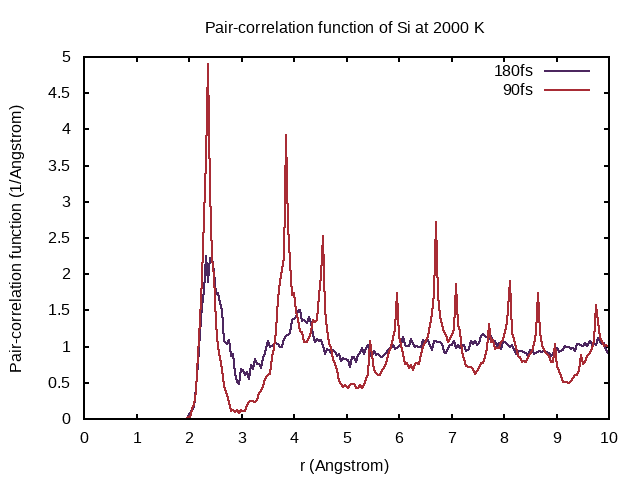
Why does the pair-correlation function at 90fs feature distinct peaks even beyond 4Å?
Click to see the answer!
In the first 90 fs, the system is still close to its crystal structure. As a crystal has long-range order distinct peaks appear in the pair-correlation function.
Also note that it makes no sense to display $g(r)$ for $r$ longer than half the shortest dimension of the supercell. That is, here $r$ should be kept below 5.4 Å.
What is the interpretation of the pair-correlation function at large distances? What is the interpretation at short distances? What is the characteristic shape of the pair-correlation function for liquids?
Visualize the liquid silicon using py4vasp!
import py4vasp
mycalc = py4vasp.Calculation.from_path( "./e02_melting-Si" )

mycalc.structure[:].plot()
The ionic positions at each step are written to the XDATCAR file. The trajectory represents the actual movement of a particle through space. For instance, in the graphic below the cyan atom moves according to the gray arrow and its trajectory leaves the central green box.
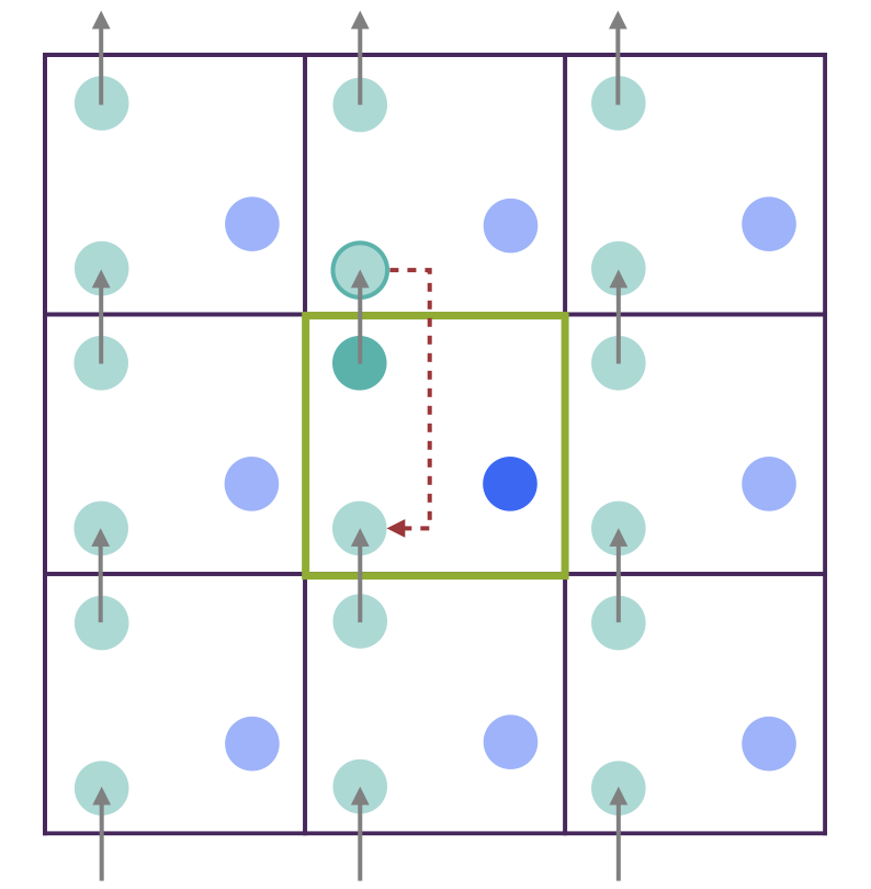
An alternative of the representation in the XDATCAR file would be the central-box representation. It is obtained by wrapping the ionic trajectories by means of applying periodic boundary conditions to the ionic positions at each time step. In the graphic, that means replacing the cyan atom with its periodic image as indicated with the red dashed arrow.
Is the volume of your MD simulation constant? What happens to an atom when passing the boundary of the unit cell in your simulation?
2.3.1 Restart an MD simulation and adjust the simulation time
Copy the latest ionic positions from CONTCAR to POSCAR and change the INCAR file to run for additional 15fs. Check the meaning of NPACO, APACO, NBLOCK and KBLOCK. You can use these tags to change the maximum distance at which the pair-correlation function is evaluated to 5.4 Å and restart from the latest ionic positions!
Click to see the answer!
In the INCAR file, set NSW = 5 and APACO = 5.4. Then, enter
cd $TUTORIALS/MD/e02_*
    mkdir restart
    cp KPOINTS POTCAR WAVECAR restart/.
    awk '!/NSW/{ print } END{ print "\nNSW    = 5\nAPACO  = 5.4"}' INCAR > restart/INCAR
    cp CONTCAR restart/POSCAR
    cd restart
    mpirun -np 2 vasp_gam
Does the new PCDAT correspond to sampling for 195 fs or 15 fs? How does this impact the quality of the pair-correlation function?
To find the answer, you can visualize the new pair-correlation function by entering the following and reopening pair_correlation.png!
cd $TUTORIALS/MD/e02_*
cp PCDAT PCDAT.195fs
bash pair_correlation.sh .195fs
gnuplot pair_correlation.gp
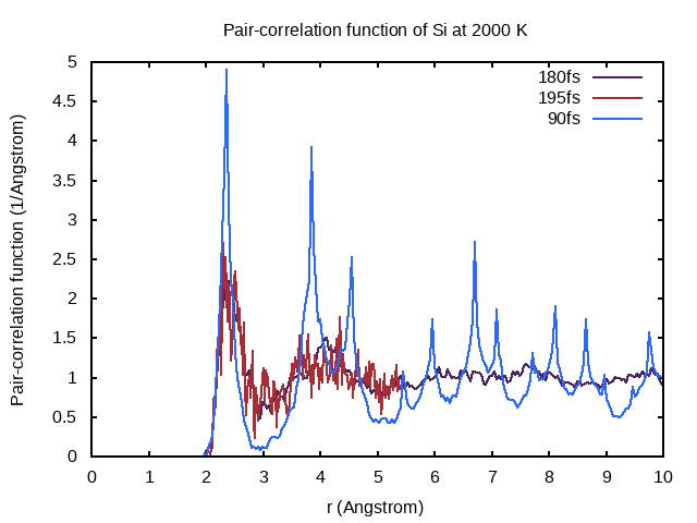
Click to see the answer!
The pair-correlation function corresponds to sampling the last 15 fs of a total simulation time of 195 fs, as you can see from the bad quality of the pair-correlation function.
2.4 Questions
- How is long-range order reflected in the pair-correlation function?
- Is the format of the CONTCAR and the POSCAR file the same? What information does the CONTCAR file contain?
- What do the tags APACO and NPACO set?
- Which output file of VASP contains the trajectories of a molecular dynamics simulations?
By the end of this tutorial, you will be able to:
- specify geometric coordinates in the ICONST file
- monitor coordinates by means of the REPORT file
- estimate the length of a simulation
- simulate an NpT ensemble using the Langevin thermostat
- create a POSCAR for a supercell without guidance
3.1 Task
Monitor the geometric coordinates during an ab-initio MD simulation of 16 silicon atoms in an NpT ensemble using the Langevin thermostat.
There are various thermostats implemented in VASP. The thermostat is set using the MDALGO tag. In the present example, we are using the Langevin thermostat with MDALGO = 3. It has both, stochastic and deterministic, terms that modify the equations of motion. The deterministic Nosé-Hoover thermostat was used in Example 1 and 2. The Andersen thermostat with MDALGO = 1 introduces temperature entirely stochastically.
For systems with strong intramolecular forces, e.g., bond stretching, the Andersen thermostat and Langevin thermostat do not introduce any extra concerns regarding ergodicity. Actually, they are quite effective at equilibrating such degrees of freedom. In contrast, the Nosé-Hoover thermostat lacks ergodicity in small or stiff systems. For instance, this is seen in the simulation of a single butane molecule. In practice, the choice of the thermostat mostly depends on the choice of the thermodynamic ensemble as implemented in VASP. Check out the possible combinations of thermostats and ensembles on the VASP Wiki!
During an MD simulation, you might want to monitor the arrangement of atoms at each time step. This arrangement of atoms broadly falls under the keyword of molecular geometry. In VASP, you can specify the internal geometric coordinates by means of the ICONST file. Check out the description on the VASP Wiki!
3.2 Input
The input files to run this example are prepared at $TUTORIALS/MD/e03_monitoring.
Create a 2x2x2 supercell of the primitive unit cell of cubic-diamond Si! Recall the commands from Example 1, add them to the code box below, and then execute it!
from pymatgen.core import Structure

my_struc = Structure.from_file("./e03_monitoring/Si_mp-149_conventional_standard.cif", primitive=True)

# make a 2x2x2 supercell of the primitive unit cell

# write supercell to POSCAR format
# with filename="./e03_monitoring/POSCAR"
Si16
1.0
  -5.4687279999999996   -5.4687279999999996    0.0000000000000000
  -5.4687279999999996    0.0000000000000000   -5.4687279999999996
   0.0000000000000003   -5.4687279999999996   -5.4687279999999996
Si
16
direct
   0.1250000000000000    0.1250000000000000    0.1250000000000000 Si
   0.1250000000000000    0.1250000000000000    0.6250000000000001 Si
   0.1250000000000001    0.6250000000000001    0.1250000000000000 Si
   0.1250000000000002    0.6250000000000000    0.6250000000000000 Si
   0.6250000000000001    0.1250000000000000    0.1250000000000000 Si
   0.6250000000000000    0.1250000000000001    0.6250000000000000 Si
   0.6250000000000000    0.6250000000000000    0.1250000000000001 Si
   0.6250000000000001    0.6250000000000000    0.6250000000000000 Si
   0.2500000000000000    0.2500000000000000    0.2500000000000000 Si
   0.2499999999999999    0.2500000000000001    0.7500000000000000 Si
   0.2499999999999999    0.7500000000000000    0.2500000000000001 Si
   0.2499999999999999    0.7500000000000001    0.7500000000000000 Si
   0.7499999999999999    0.2500000000000000    0.2500000000000000 Si
   0.7499999999999999    0.2500000000000001    0.7500000000000000 Si
   0.7499999999999999    0.7500000000000000    0.2500000000000001 Si
   0.7499999999999998    0.7500000000000000    0.7500000000000001 Si
SYSTEM = Si16
ISYM   = 0        ! no symmetry imposed

! ab initio
PREC   = Normal
IVDW   = 10

ISMEAR = -1      ! Fermi smearing
SIGMA  = 0.0258  ! smearing in eV

ENCUT  = 300
EDIFF  = 1e-6

LWAVE  = F
LCHARG = F

LREAL  = F

! MD
IBRION = 0        ! MD (treat ionic degrees of freedom)
NSW    = 10       ! no of ionic steps
POTIM  = 2.0      ! MD time step in fs

MDALGO = 3                ! Langevin thermostat
LANGEVIN_GAMMA   = 1      ! friction
LANGEVIN_GAMMA_L = 10     ! lattice friction
PMASS  = 10               ! lattice mass
TEBEG  = 400              ! temperature

ISIF   = 3        ! update positions, cell shape and volume
LR 1 7
LR 2 7
LR 3 7
LA 2 3 7
LA 1 3 7
LA 1 2 7
LV 7
Not only Gamma point
 0
Gamma
 2 2 2
 0 0 0
Pseudopotentials of Si.
In the INCAR file, the use of spacegroup symmetry in the entire calculation is switched off with ISYM=0. In the DFT steps, the precision is set to normal using the PREC tag and van der Waals corrections are considered with IVDW. Besides other common parameters set for DFT calculations, we switch of writing the WAVECAR and CHGCAR files.
Tags regarding MD steps include IBRION, NSW, and POTIM. Recall their meaning! Additionally, ISIF=3 and MDALGO=3 selects the NpT ensemble employing the Langevin thermostat. Check out the related tags on the VASP Wiki!
The ICONST file specifies a number of geometric coordinates that are monitored. The first column defines the kind of geometric coordinate, e.g., the distance of an ion to the origin, or an angle. The following integers refer to the atoms in the same order as defined in the POSCAR file. That is except for the last integer, which specifies the action, i.e., 7 defines monitoring.
The KPOINTS file defines a uniform $\mathbf{k}$ mesh spanning two reciprocal lattice vectors in each direction including the Gamma point. It would be preferable to use a larger unit cell instead but this is computationally expensive. In practice, you need to check whether the quantity of interest is converged with respect to the size of the unit cell and number of $\mathbf{k}$ points. Here, we merely monitor some geometric coordinates, so the settings are adequate.
3.3 Calculation
Open a terminal, navigate to this example's directory and run VASP by entering the following:
cd $TUTORIALS/MD/e03_*
mpirun -np 4 vasp_std
Note, that here you need to use the executable vasp_std instead of vasp_gam. Why is that?
Click to see the answer!
The executable vasp_gam can only be used for calculations considering a single $\mathbf{k}$ point, that is the Gamma point, because VASP internally considers some arrays to contain real numbers instead of complex numbers. Here, the KPOINTS file defines a uniform $\mathbf{k}$ mesh, i.e., more than just the Gamma point.
Open the REPORT file and find the monitored coordinates in each MD step!
For instance, in the first MD you will find
========================================
         MD step No.       1
========================================

  Atomic velocities initialized by STEP_tb

  >Monit_coord
   mc> LR         7.73395
   mc> LR         7.73395
   mc> LR         7.73395
   mc> LA         1.04720
   mc> LA         1.04720
   mc> LA         1.04720
   mc> LV       327.10634

  Lattice velocities initialized by STEP_tb

   t_b>    400.000    396.375    212.541    367.348

  >Energies
                    E_tot             E_pot             E_kin               EPS                ES
   e_b>   -0.87877738E+02   -0.88779929E+02    0.90219107E+00    0.00000000E+00
    0.00000000E+00

           RANDOM_SEED =         414621889              228                0
Extract the monitored volume and plot it!
! cat ./e03_monitoring/REPORT | grep "mc> LV" > ./e03_monitoring/monitored_cell_volume.dat

import numpy as np
from py4vasp import plot

volume = np.loadtxt("./e03_monitoring/monitored_cell_volume.dat", usecols=2)

# plot the volume
plot(np.arange(len(volume))+1, volume, "relaxation", xlabel="Number of MD steps", ylabel="Volume (ų)")
Open the OUTCAR file and find the elapsed time! How long did the completion of 10 ab-initio MD steps take? Use this result to estimate the computational time necessary to generate a MD trajectory of 10000 MD steps!
Click to see the answer!
Depending on the exact hardware and computational setup, these 10 MD steps take roughly 74 s. Then, 10000 MD steps take more than 20 h!
10000 MD steps is a typical number of steps necessary to deduce anything reasonable from an MD simulation. Therefore, this example shows that ab-initio MD simulations are computationally expensive and time-consuming. This renders ab-initio MD infeasible for many systems.
3.4 Questions
- What does a line that reads
R 1 6 0in the ICONST file define? - How can the computational time of a long MD simulation be estimated?
- What does the LANGEVIN_GAMMA tag specify?